Example 2 - CMAP

The purpose of example 2 in the lower right portion of Figure 1 in the application note manuscript was to exemplify use of the CMAP packaged dataset, along with user supplied and built-in phenotypic metrics. An interactive Jupyter notebook (Jupyter core version 4.9.1) was used to carry out this analysis with version Python 3.9.5, Phenonaut version 1.0.0, Numpy version 1.20.3, Pandas version 1.4.0, scikit-learn version 0.24.2, and PyTorch version 1.10.2 installed. The notebook can be found in the Phenonaut source repository named “example2_CMAP_metric_groups.ipynb”. The notebook was used to evaluate the built in (Euclidean and Manhattan distances) and user defined phenotypic metrics (TCCS[6] and scalar projection[7]). In this notebook, the CMAP packaged dataset loader is used to obtain a copy of the public CMAP dataset, which is then filtered, keeping only CRISPR perturbation repeats on the A549 cell line transfected with the pLX311-Cas9 vector, from here referred to using the internal CMAP nomenclature of the ‘A549.311’ cell line. The phenotypic metrics are then evaluated using Area Under the Receiver Operator Characterstic Curve (AUROC) metric, indicating their ability to group together repeats. Boxplots of the AUROC performance across repeats are then generated to give an overview of metric performance. The jupyter file “example2_CMAP_metric_groups.ipynb” available in the “Supplemental Data from Object Store” section gives the code listing required to explore and generate the boxplot shown within Figure 1 of the manuscript. A walkthrough of the notebook follows:

CRISPR (xpr) repeats present in the CMAP dataset offer the possibility to evaluate phenotypic metrics applied to different representations of the level 5 L1000 profiles within the CMAP dataset. Here, we evaluate metric-feature space pairs and their ability to correctly rank xpr repeats as highly similar to each other. Metric and feature space pairs are scored through evaluation of the area under receiver operating characteristic (AUROC), with 0.5 representative of random guessing, 1, perfect performance, and 0 representative of perfectly incorrect ranking being applied to xpr repeats. We now use the CMAP package dataset loader to extract the A549.311 cell line and perform the evaluation of the following phenotypic metrics:

• Euclidean distance

• Manhattan/cityblock distance

• Cosine similarity

• Scalar projection

We evaluate these on:

• Full feature space

• Standard Scalar feature space

• PCA feature space

• t-SNE feature space

• UMAP feature space.

t-SNE and UMAP are unsuitable for the application of the cosine similarity and scalar projection, being angular metrics and are not applied.

First, use the Phenonaut CMAP dataloader to load the entire CMAP dataset. Process it, extracting the A549.311 cell line where treatment is “xpr peturbation” or “ctl_untrt”. Once processed, save it in a pickle so that it can more quickly be loaded in the future. As a “standard scaler” feature space is required for input to PCA, UMAP and t-SNE, we generate standard scalar dataset. Next, we define the similarity metrics and scoring function. In the code below, BASE_PROJECT_DIR took the location of a convenient output directory on the local filesystem.

import numpy as np
import pandas as pd
import phenonaut, phenonaut.transforms
from pathlib import Path
BASE_PROJECT_DIR=Path("projects/cmap")
if not BASE_PROJECT_DIR.exists():
    BASE_PROJECT_DIR.mkdir(parents=True)
phe_object_path=BASE_PROJECT_DIR/"phe_ob_cmap_trt_xpr_A549.311.pickle.gz"
if not phe_object_path.exists():
    cmap_data=phenonaut.packaged_datasets.CMAP("/local_scratch/data/phenonaut_datasets/cmap")
    phe=phenonaut.Phenonaut(cmap_data['ds'])

    phe.new_dataset_from_query("xpr", "cell_id=='A549.311' and (pert_type=='trt_xpr' or pert_type=='ctl_untrt')", "cmap")
    phe['xpr'].perturbation_column="pert_iname"
    phe.save(phe_object_path)
phe=phenonaut.Phenonaut.load(phe_object_path)
phe.clone_dataset("xpr", "xpr_scaled",overwrite_existing=True)
phenonaut.transforms.StandardScaler()(phe['xpr_scaled'])
from scipy.spatial.distance import cosine as cosine_distance
from dataclasses import dataclass
from typing import Union, Callable

@dataclass
class PhenotypicMetric:
    name: str
    func: Union[str, Callable]
    lower_is_better: bool = True
    is_angular: bool = False
metrics = [
    PhenotypicMetric("random", lambda x, y: np.random.uniform(0, 1)),
    PhenotypicMetric("euclidean", "euclidean"),
    PhenotypicMetric("Manhattan", "cityblock"),
    PhenotypicMetric("cosine similarity", lambda x, y: 1 - cosine_distance(x, y), lower_is_better = False, is_angular=True),
    PhenotypicMetric("scalar projection", phenonaut.metrics._scalar_projection_scaled, lower_is_better = False, is_angular=True),
]
metrics_dictionary = {m.name: m for m in metrics}

from sklearn.metrics import roc_auc_score
def auroc_scores_for_perturbation_repeats(ds:phenonaut.data.Dataset, metric:PhenotypicMetric, average_repeats:bool=True)->tuple:
    pert_scores=[]
    df_dict = {"score": [], "perturbation": []}
    dist_mat = ds.distance_df(
        ds,
        metric=metric.func,
        lower_is_better=metric.lower_is_better,
    ).values
    for pert_name in ds.df[ds.perturbation_column].unique():
        pert_indexes = [ds.df.index.get_loc(idx) for idx in ds.df.query(f"pert_iname == '{pert_name}'").index]
        repeat_scores = []
        if metric.lower_is_better:
            for pert_index in pert_indexes:
                predictions = np.zeros(dist_mat.shape[1], dtype=int)
                predictions[pert_indexes] = 1
                prediction_score = -dist_mat[pert_index, :]
                rocscore = roc_auc_score(predictions, prediction_score)
                repeat_scores.append(rocscore)
        else:
            for pert_index in pert_indexes:
                predictions = np.zeros(dist_mat.shape[1], dtype=int)
                predictions[pert_indexes] = 1
                prediction_score = dist_mat[pert_index, :]
                rocscore = roc_auc_score(predictions, prediction_score)
                repeat_scores.append(rocscore)
        if average_repeats:
            df_dict['score'].append(np.mean(repeat_scores))
            df_dict['perturbation'].append(pert_name)
        else:
            df_dict['score'].extend(repeat_scores)
            df_dict['perturbation'].extend([pert_name]*len(repeat_scores))
        pert_scores.append(np.mean(repeat_scores))
    return pert_scores, pd.DataFrame(df_dict)

Next, we generate PCA, UMAP, t-SNE using the standard scalar feature space. ndims = 2 at this stage so we can obtain a unoptimized baseline.

In order to perform a sanity check, the xpr repeats were visualised in PCA, tSNE and UMAP space.

Producing the following figures:

PCA scatter of CMAP A549.311 cell line CRISPR repeats. Large blue ‘+’ are untreated controls.

UMAP scatter of CMAP A549.311 cell line CRISPR repeats. Large blue ‘+’ are untreated controls.

t-SNE scatter of CMAP A549.311 cell line CRISPR repeats. Large blue ‘+’ are untreated controls.

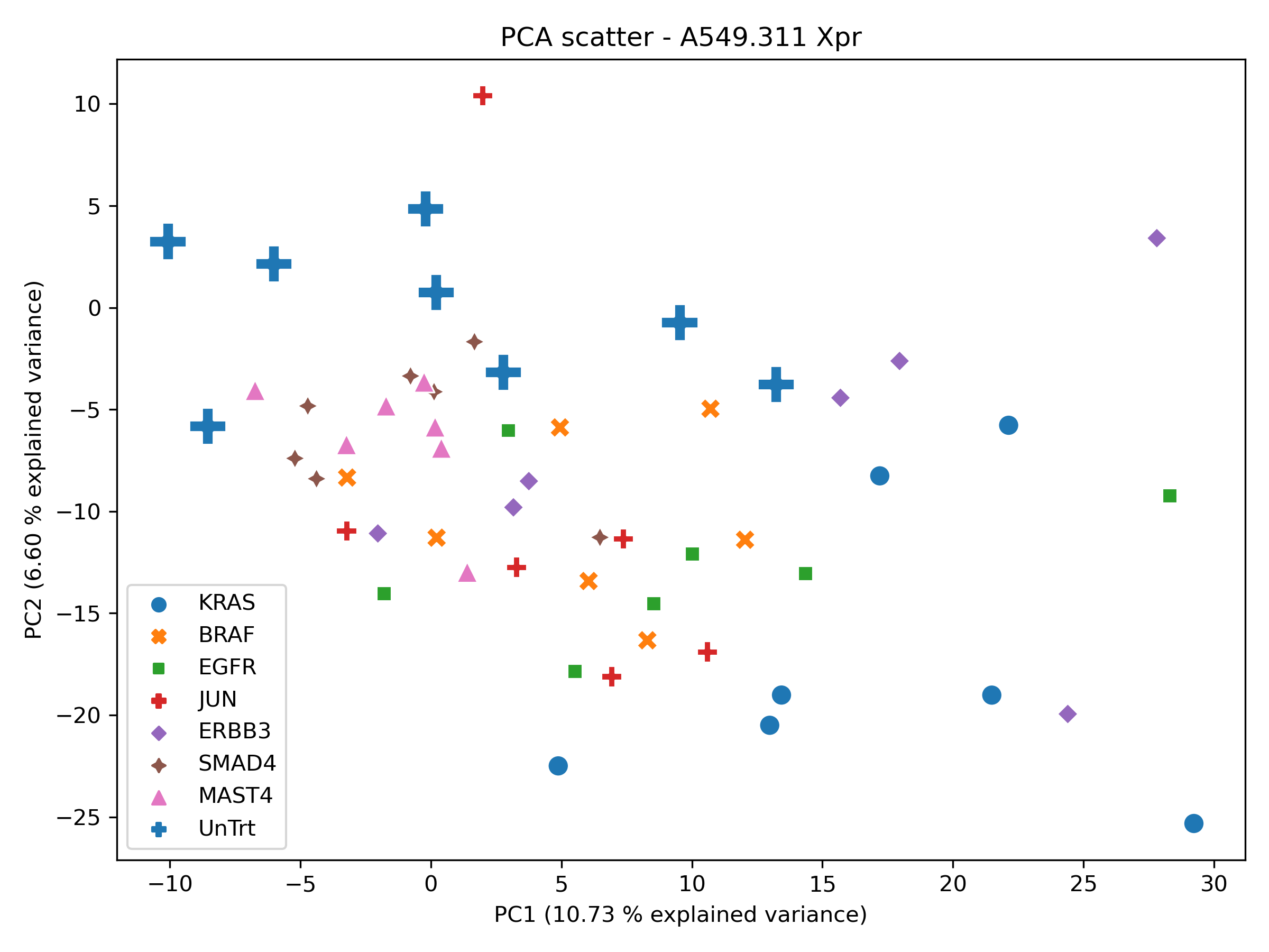
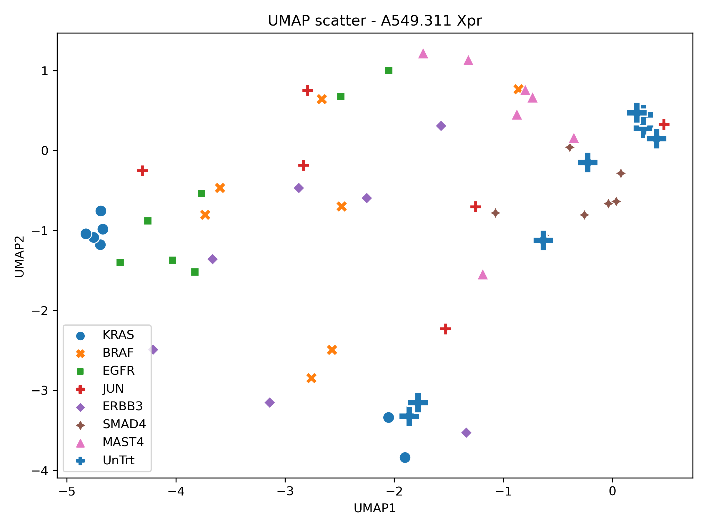
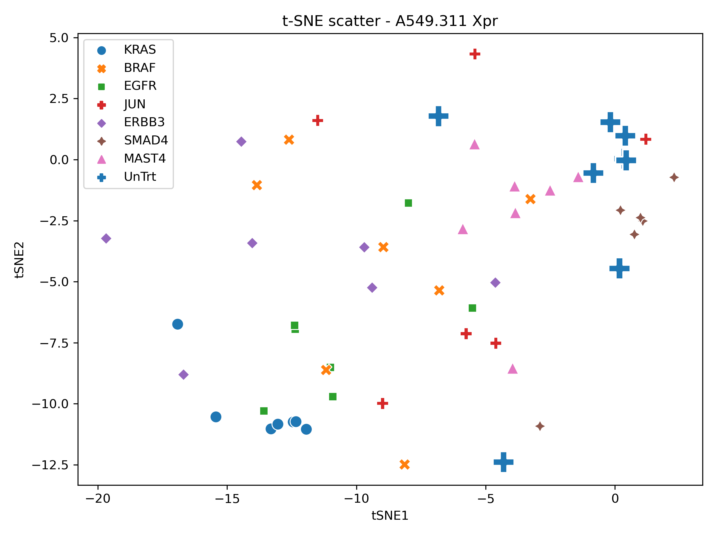
With local structure present within the UMAP and tSNE scatters for a selection of xpr perturbations which roughly group together, the dataset was deemed appropriate for phenotypic metric performance evaluation.

The following code is used to generate AUROC scores across xpr repeats for appropriate feature space-metric pairs:

if (BASE_PROJECT_DIR/"metric_scores.csv").exists():
    raise FileExistsError(f"{BASE_PROJECT_DIR}/metric_scores.csv exists")

perturbation_scores_df=pd.DataFrame()
for features_name, ds_name in zip(
    ("Full", "Std", "PCA", "UMAP", "t-SNE"),
    ("xpr", "xpr_scaled", "xpr_scaled_pca", "xpr_scaled_umap", "xpr_scaled_tsne"),
):
    print(f"Working on {features_name}")
    for metric in metrics:
        if metric.is_angular and features_name in ['UMAP','t-SNE']:
            continue
        print(f"{metric.name=}")
        scores, feature_metric_df=auroc_scores_for_perturbation_repeats(phe[ds_name],metric)
        feature_metric_df["metric_name"]=metric.name
        feature_metric_df["features"]=features_name
        perturbation_scores_df=pd.concat([perturbation_scores_df, feature_metric_df]).reset_index(drop=True)
perturbation_scores_df.to_csv(BASE_PROJECT_DIR/"metric_scores.csv")

A boxplot was then generated to summarise the results of the above metric evaluation. Whilst distance measurements in UMAP and TSNE space should be avoided due to their dependence on hyperparameters, this is performed for demonstration purposes:

import matplotlib.pyplot as plt
import seaborn as sns

metric_scores_df=pd.read_csv(BASE_PROJECT_DIR/"metric_scores.csv")

fig, ax = plt.subplots(1, facecolor='w')
# the size of A4 paper
fig.set_size_inches(12.0, 8)
sns.boxplot(
    data=metric_scores_df,
    y="score",
    x="metric_name",
    hue="features",
    ax=ax,
    showmeans=True,
    meanprops={"marker": "o", "markerfacecolor": "white", "markeredgecolor": "black", "markersize": "10"},
)
ax.axhline(0.5, color="black", linestyle="--")
ax.set(ylim=(0.2,1), xlabel='Metric', ylabel='AUROC', title="AUROC scores of average xpr repeat reproducibility across phenotypic metrics and feature spaces")

plt.tight_layout()
fig.savefig(BASE_PROJECT_DIR/"boxplot.png", dpi=300)

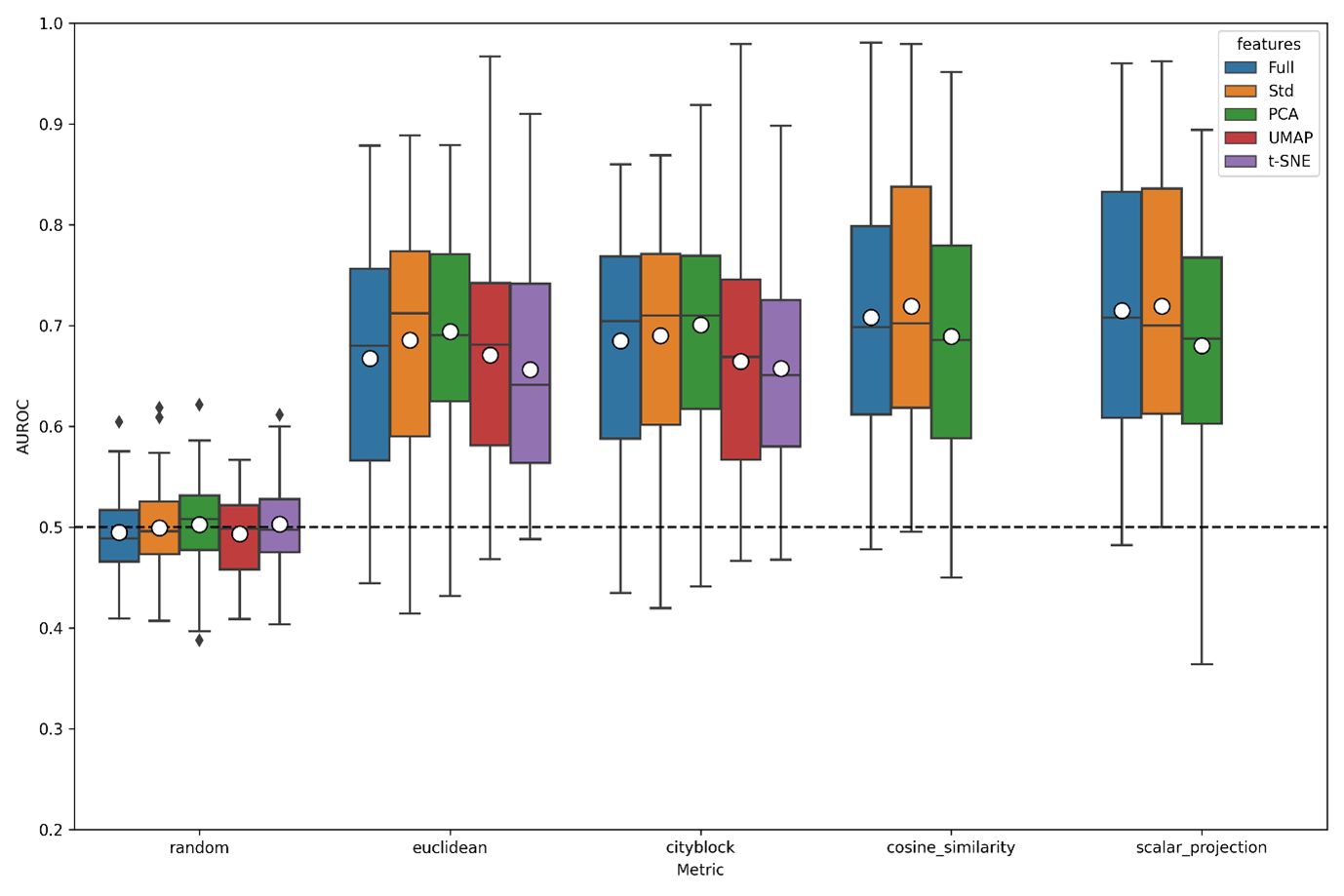
Resulting in the following figure:

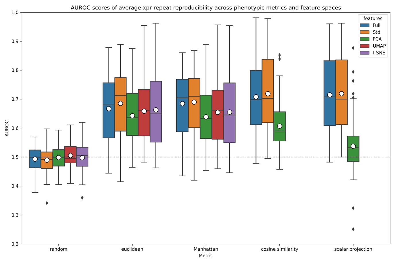
Boxplot of AUROC scores across averaged xpr repeats of the A549.311 cell line within CMAP. For each dimensionality reduction technique (PCA, UMAP and tSNE), 2 dimensions were requested, and all other options kept to default settings.

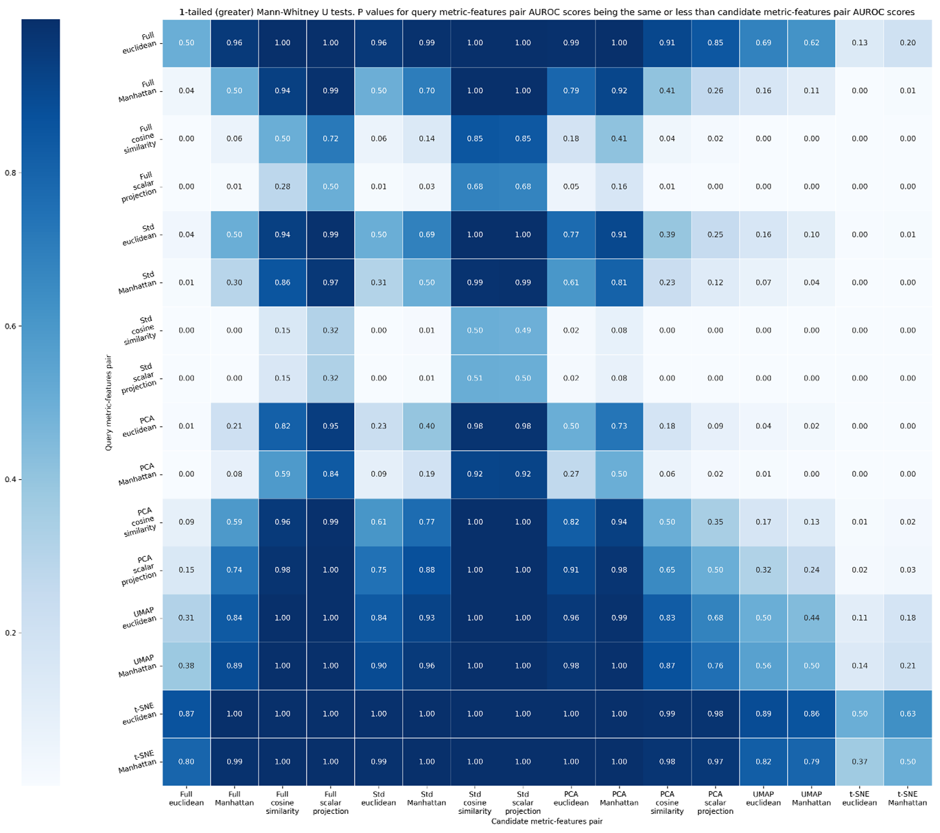
The above figure gives us an insight into metric-feature space performance, but statistically testing all distributions against the others will allow us to recommend a metric-feature space pair. For this, we use the Mann-Whitney U rank test in a 1-tailed mode, testing the alternative hypothesis that a distribution is stochastically greater than the other. This produces a matrix as shown in Figure S7, and summarised in Figure S8. Once calculated, two representative heatmaps can be generated.

from copy import deepcopy
metric_scores_df=pd.read_csv(BASE_PROJECT_DIR/"metric_scores.csv")
@dataclass
class FeatureSpaceAndMetric():
    featurespace:str
    metric:PhenotypicMetric
from scipy.stats import mannwhitneyu
featurespeace_metric_combinations=[FeatureSpaceAndMetric(feature_space, metric) for feature_space in ("Full", "Std", "PCA", "UMAP", "t-SNE") for metric in [m for m in metrics if m.name !="random"] if not (metric.is_angular and feature_space in ['UMAP', 't-SNE'])]

pvals=np.full((len(featurespeace_metric_combinations), len(featurespeace_metric_combinations)),np.nan)

for i1, fsm1 in enumerate(featurespeace_metric_combinations):
    for i2, fsm2 in enumerate(featurespeace_metric_combinations):
        vals1=metric_scores_df.query(f"features=='{fsm1.featurespace}' and metric_name=='{fsm1.metric.name}'")['score'].values
        vals2=metric_scores_df.query(f"features=='{fsm2.featurespace}' and metric_name=='{fsm2.metric.name}'")['score'].values
        pvals[i1, i2]=mannwhitneyu(vals1, vals2,alternative="greater").pvalue
mwu_df=pd.DataFrame(data=pvals, columns=[f"{fsm.featurespace} {fsm.metric.name}" for fsm in featurespeace_metric_combinations], index=[f"{fsm.featurespace} {fsm.metric.name}" for fsm in featurespeace_metric_combinations])
from phenonaut.output import write_heatmap_from_df
write_heatmap_from_df(mwu_df,"1-tailed (greater) Mann-Whitney U tests. P values for query metric-features pair AUROC scores being the same or less than candidate metric-features pair AUROC scores", BASE_PROJECT_DIR/"mwu-heatmap.png", figsize=(20,16), lower_is_better=True, highlight_best=False, put_cbar_on_left=True, axis_labels=("Candidate metric-features pair A", "Query metric-features pair"))
better_than_count=np.sum(pvals[:]<0.05,axis=1)
better_than_count=np.insert(better_than_count,-2, [0,0])
better_than_count=np.insert(better_than_count,better_than_count.shape[0], [0,0]).reshape(5,4)
better_than_df=pd.DataFrame(data=better_than_count, index=("Full", "Std", "PCA", "UMAP", "t-SNE"), columns=[m.name for m in metrics if m.name !="random"])
custom_annotation=deepcopy(better_than_df)
custom_annotation.loc[['UMAP','t-SNE'], ['scalar projection', 'cosine similarity']]="NA"
write_heatmap_from_df(better_than_df,"Num significant at 0.05 level", BASE_PROJECT_DIR/"mwu-betterthan-heatmap.png", figsize=(5,4), lower_is_better=False, annotation_format_string_value="g", annot=custom_annotation.transpose().values, sns_colour_palette="Blues")

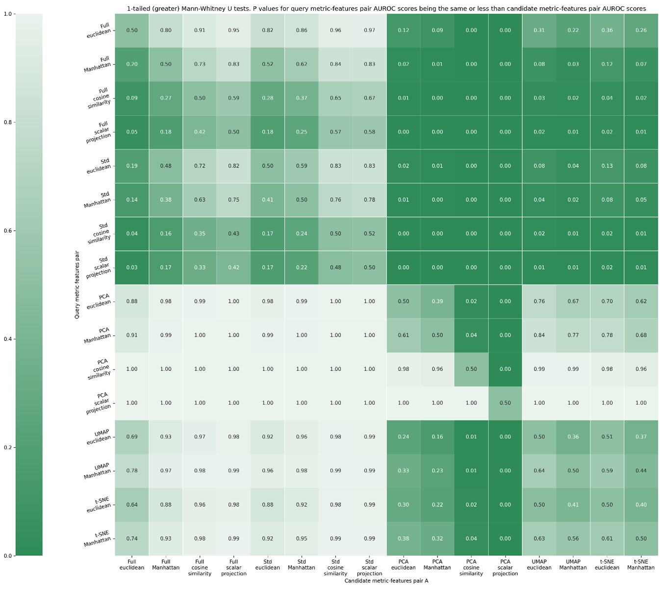
1-tailed Mann Whitney-U (greater than) test, evaluating if the query metric-feature space combination is better than the candidate-feature space combination. Values denote p-values that the metric-feature space combination in a given row is performed better than the metric-feature space column given in the column by chance along. If this value is <0.05, we deem there to be a less than 5 % chance that the metric-feature space combination outperformed the other by chance.

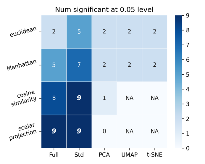
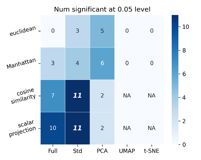
Counts of the number of features-space metric pairs that were significantly better performing than other metric-feature space pairs. Suggests that scalar projection applied to full and standard scalar feature space outperforms the same number of metric-feature space pairs as cosine similarity applied to standard scalar feature space.

Whilst the above shows that scalar projection applied to full and standard scalar feature space outperforms the same number of metric-feature space pairs as cosine similarity applied to standard scalar feature space, there is no significant (at the 0.05 level) performance difference between any of those top metric-feature space combinations, as evidenced in Figure S7. Additionally, the PCA, UMAP and t-SNE feature spaces are in 2 dimensions only. This can be optimised using a simple scanning approach to reach optimum AUROC scores for each metric-feature space pair.

from dataclasses import dataclass
from phenonaut.transforms.dimensionality_reduction import PCA,TSNE,UMAP
from typing import Union, Callable
import matplotlib.pyplot as plt
import seaborn as sns
from enum import Enum, auto
from copy import deepcopy
ndims_scan_csv_file=BASE_PROJECT_DIR/"res_ndims_scan.csv"

if not ndims_scan_csv_file.exists():

    def eval_all_metrics(sds, num_dimensions):
        print(f"{num_dimensions=}")
        center_on_perturbation = "UnTrt"
        pca_ds=deepcopy(sds)
        PCA()(pca_ds, ndims=num_dimensions, center_on_perturbation_id=center_on_perturbation)
        tsne_ds=deepcopy(sds)
        TSNE()(tsne_ds, ndims=num_dimensions, center_on_perturbation_id=center_on_perturbation)
        umap_ds=deepcopy(sds)
        UMAP()(umap_ds, ndims=num_dimensions, center_on_perturbation_id=center_on_perturbation)
        results=np.empty((len([m for m in metrics if m.name != "random"]), 3))

        for i, metric in enumerate([m for m in metrics if m.name != "random"]):
            for j, (ds, angular_is_ok) in enumerate(((pca_ds, True), (tsne_ds, False), (umap_ds, False))):
                if not metric.is_angular or (metric.is_angular and angular_is_ok):
                    auroc_scores, _ = auroc_scores_for_perturbation_repeats(ds,metric)
                    results[i,j]=np.mean(auroc_scores)
                else:
                    results[i,j]=np.nan
        return results

    from copy import deepcopy
    from multiprocessing import Pool


    sds = deepcopy(phe["xpr_scaled"])

    n_dims_list = np.arange(2, min(sds.df.shape[0]-2, sds.df.shape[1]-2))
    print(f"{len(n_dims_list)=}")
    # [PCA, tSNE, UMAP], metric, dimensions
    pool = Pool()
    res = np.array(pool.starmap(eval_all_metrics, ((sds, nd) for nd in n_dims_list)))
    pool.close() # ATTENTION HERE

    df_metric_list=[]
    df_features_list=[]
    df_ndims_list=[]
    df_score_list=[]

    for i in range(res.shape[0]):
        for j in range(res.shape[1]):
            for k in range(res.shape[2]):
                print(i,j,k)
                df_ndims_list.append(i+2)
                df_metric_list.append([m for m in metrics if m.name != "random"][j].name)
                df_features_list.append(["PCA", "tSNE", "UMAP"][k])
                df_score_list.append(res[i,j,k])

    import pandas as pd
    pd.DataFrame({"metric":df_metric_list, "features":df_features_list, "ndims":df_ndims_list, "score":df_score_list}).to_csv(ndims_scan_csv_file)
# CSV file exists or has been generated above
ndims_df=pd.read_csv(ndims_scan_csv_file)

fig, ax=plt.subplots(1,3, figsize=(16,7), sharey=True)
sns.scatterplot(data=ndims_df.query('features=="PCA"'), x='ndims', y="score", style='metric', hue='metric', ax=ax[0], legend=True)
ax[0].title.set_text('PCA - ndims vs AUROC score')
sns.scatterplot(data=ndims_df.query('features=="UMAP" and metric!="cosine similarity" and metric!="scalar projection"'), x='ndims', y="score", style='metric', hue='metric', ax=ax[1], legend=True)
ax[1].title.set_text('UMAP - ndims vs AUROC score')
sns.scatterplot(data=ndims_df.query('features=="tSNE" and metric!="cosine similarity" and metric!="scalar projection"'), x='ndims', y="score", style='metric', hue='metric', ax=ax[2],legend=True)
ax[2].title.set_text('t-SNE - ndims vs AUROC score')
lines_labels = [ax.get_legend_handles_labels() for ax in fig.axes]
lines, labels = [sum(lol, []) for lol in zip(*lines_labels)]
for axis in ax: sns.move_legend(axis, "lower right")
plt.tight_layout()
fig.savefig(BASE_PROJECT_DIR/"ndims_optimisation_scatter.png", dpi=300)

Producing the following:

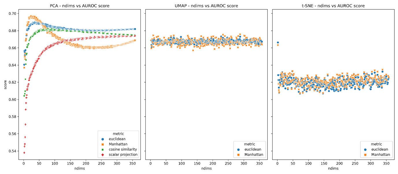
AUROC scores for PCA, UMAP and t-SNE feature spaces across a range of dimensions for each appropriate metric.

The top performing ndims for each metric-feature space are summarised in the table below.

Optimal number of dimensions (maximising AUROC scores) for each metric-feature space pair (AUROC).

Metric	PCA optimized ndims	UMAP optimized ndims	t-SNE optimized ndims
Euclidean	36	227	2
Manhattan	24	288	2
Cosine similarity	78	NA	NA
Scalar projection	356	NA	NA

With the optimum number of dimensions for metric-feature space pairs determined, we may calculate AUROC scores again.

metric_scores = {"metric_name": [], "score": [], "features": []}
metrics_dict = {m.name: m for m in metrics}
perturbation_scores_ndim_opt=pd.DataFrame()

print(metrics_dict)
ds_pca_36 = deepcopy(phe["xpr_scaled"])
PCA()(ds_pca_36, ndims=36, center_on_perturbation_id=center_on_perturbation)
ds_pca_24 = deepcopy(phe["xpr_scaled"])
PCA()(ds_pca_24, ndims=24, center_on_perturbation_id=center_on_perturbation)
ds_pca_78 = deepcopy(phe["xpr_scaled"])
PCA()(ds_pca_78, ndims=78, center_on_perturbation_id=center_on_perturbation)
ds_pca_356 = deepcopy(phe["xpr_scaled"])
PCA()(ds_pca_356, ndims=356, center_on_perturbation_id=center_on_perturbation)

ds_tsne_2 = deepcopy(phe["xpr_scaled"])
TSNE()(ds_tsne_2, ndims=2)

ds_umap_227 = deepcopy(phe["xpr_scaled"])
UMAP()(ds_umap_227, ndims=227)
ds_umap_288 = deepcopy(phe["xpr_scaled"])
UMAP()(ds_umap_288, ndims=288)

for features_name, ds, metric in [
    ("Full", deepcopy(phe["xpr"]), metrics_dict["random"]),
    ("Std", deepcopy(phe["xpr_scaled"]), metrics_dict["random"]),
    ("PCA", ds_pca_24, metrics_dict["random"]),
    ("UMAP", ds_umap_227, metrics_dict["random"]),
    ("t-SNE", ds_tsne_2, metrics_dict["random"]),
    ("Full", deepcopy(phe["xpr"]), metrics_dict["euclidean"]),
    ("Std", deepcopy(phe["xpr_scaled"]), metrics_dict["euclidean"]),
    ("PCA", ds_pca_36, metrics_dict["euclidean"]),
    ("UMAP", ds_umap_227, metrics_dict["euclidean"]),
    ("t-SNE", ds_tsne_2, metrics_dict["euclidean"]),
    ("Full", deepcopy(phe["xpr"]), metrics_dict["Manhattan"]),
    ("Std", deepcopy(phe["xpr_scaled"]), metrics_dict["Manhattan"]),
    ("PCA", ds_pca_24, metrics_dict["Manhattan"]),
    ("UMAP", ds_umap_288, metrics_dict["Manhattan"]),
    ("t-SNE", ds_tsne_2, metrics_dict["Manhattan"]),
    ("Full", deepcopy(phe["xpr"]), metrics_dict["cosine similarity"]),
    ("Std", deepcopy(phe["xpr_scaled"]), metrics_dict["cosine similarity"]),
    ("PCA", ds_pca_78, metrics_dict["cosine similarity"]),
    ("Full", deepcopy(phe["xpr"]), metrics_dict["scalar projection"]),
    ("Std", deepcopy(phe["xpr_scaled"]), metrics_dict["scalar projection"]),
    ("PCA", ds_pca_356, metrics_dict["scalar projection"]),
]:
    print(f"Working on {features_name}")
    scores, feature_metric_df=auroc_scores_for_perturbation_repeats(ds,metric)
    feature_metric_df["metric_name"]=metric.name
    feature_metric_df["features"]=features_name
    perturbation_scores_ndim_opt=pd.concat([perturbation_scores_ndim_opt, feature_metric_df]).reset_index(drop=True)

perturbation_scores_ndim_opt.to_csv(BASE_PROJECT_DIR / "optimised_perturbation_scores_ndim_opt.csv")

and visualise:

import matplotlib.pyplot as plt
import seaborn as sns

data = pd.read_csv(BASE_PROJECT_DIR / "optimised_perturbation_scores_ndim_opt.csv")

# data['score']=data['score'].clip(upper=12000)
fig, ax = plt.subplots(1, facecolor='w')
# the size of A4 paper
fig.set_size_inches(12.0, 8)
sns.boxplot(
    data=data,
    y="score",
    x="metric_name",
    hue="features",
    ax=ax,
    showmeans=True,
    meanprops={"marker": "o", "markerfacecolor": "white", "markeredgecolor": "black", "markersize": "10"},
)
ax.axhline(0.5, color="black", linestyle="--")
data.to_csv(BASE_PROJECT_DIR/"scores.csv")
ax.set(ylim=(0.2,1), xlabel='Metric', ylabel='AUROC')
plt.tight_layout()
fig.savefig(BASE_PROJECT_DIR/"boxplot_opt.png", dpi=300)

Boxplot of AUROC scores across averaged xpr repeats of the A549.311 cell line within CMAP. For each dimensionality reduction technique (PCA, UMAP and tSNE), the optimum number of dimensions were used to maximise AUROC scores, indicating the throretical maximum scores achievable using these metric-feature space pairs, other options kept to default settings.

Similarly to before, we may repeat the statistical testing to evaluate metric-feature space pair performance with each other.

from scipy.stats import mannwhitneyu

from copy import deepcopy
optimised_perturbation_scores_df=pd.read_csv(BASE_PROJECT_DIR/"optimised_perturbation_scores.csv")
@dataclass
class FeatureSpaceAndMetric():
    featurespace:str
    metric:PhenotypicMetric
from scipy.stats import mannwhitneyu
featurespeace_metric_combinations=[FeatureSpaceAndMetric(feature_space, metric) for feature_space in ("Full", "Std", "PCA", "UMAP", "t-SNE") for metric in [m for m in metrics if m.name !="random"] if not (metric.is_angular and feature_space in ['UMAP', 't-SNE'])]

pvals=np.full((len(featurespeace_metric_combinations), len(featurespeace_metric_combinations)),np.nan)

for i1, fsm1 in enumerate(featurespeace_metric_combinations):
    for i2, fsm2 in enumerate(featurespeace_metric_combinations):
        vals1=optimised_perturbation_scores_df.query(f"features=='{fsm1.featurespace}' and metric_name=='{fsm1.metric.name}'")['score'].values
        vals2=optimised_perturbation_scores_df.query(f"features=='{fsm2.featurespace}' and metric_name=='{fsm2.metric.name}'")['score'].values
        pvals[i1, i2]=mannwhitneyu(vals1, vals2,alternative="greater").pvalue
mwu_df=pd.DataFrame(data=pvals, columns=[f"{fsm.featurespace} {fsm.metric.name}" for fsm in featurespeace_metric_combinations], index=[f"{fsm.featurespace} {fsm.metric.name}" for fsm in featurespeace_metric_combinations])
from phenonaut.output import write_heatmap_from_df
#write_heatmap_from_df(mwu_df,"1-tailed (greater) Mann-Whitney U", BASE_PROJECT_DIR/"mwu_heatmap_opt.png", figsize=(20,16), lower_is_better=True, highlight_best=False)
write_heatmap_from_df(mwu_df,"1-tailed (greater) Mann-Whitney U tests. P values for query metric-features pair AUROC scores being the same or less than candidate metric-features pair AUROC scores", BASE_PROJECT_DIR/"mwu-heatmap.png", figsize=(20,16), lower_is_better=True, highlight_best=False, put_cbar_on_left=True, axis_labels=("Candidate metric-features pair", "Query metric-features pair"), sns_colour_palette="Blues")

better_than_count=np.sum(pvals[:]<0.05,axis=1)
better_than_count=np.insert(better_than_count,-2, [0,0])
better_than_count=np.insert(better_than_count,better_than_count.shape[0], [0,0]).reshape(5,4)
better_than_df=pd.DataFrame(data=better_than_count, index=("Full", "Std", "PCA", "UMAP", "t-SNE"), columns=[m.name for m in metrics if m.name !="random"])
custom_annotation=deepcopy(better_than_df)
custom_annotation.loc[['UMAP','t-SNE'], ['scalar projection', 'cosine similarity']]="NA"
write_heatmap_from_df(better_than_df,"Num significant at 0.05 level", BASE_PROJECT_DIR/"betterthan_heatmap_opt.png", figsize=(5,4), lower_is_better=False, annotation_format_string_value="g", annot=custom_annotation.transpose().values, sns_colour_palette="Blues")

1-tailed Mann Whitney-U (greater than) test, evaluating if the query metric-feature space combination is better than the candidate-feature space combination, dimensionality reduction techniques using optimum number of dimensions to reflect theoretical maximum performance. Values denote p-values that the metric-feature space combination is a given row is performed better than the metric-feature space column given in the column by chance along. If this value is <0.05, we deem there to be a less than 5 % chance that the metric-feature space combination outperformed the other by chance.

Counts of the number of features-space metric pairs that were significantly better performing than other metric-feature space pairs. Suggests that scalar projection applied to full and standard scalar feature space outperforms other metrics, however the previous figure shows there is not a significant performance gain (0.05 level) in using the scalar projection over cosine similarity for full and standard scalar feature spaces.